Article Text

Abstract
Objective: To examine the variation between hospitals in rates of severe intraventricular haemorrhage (IVH) in preterm babies adjusting for case mix and sampling variability.
Design: Cross sectional study of pooled data from 1995 to 1997.
Setting: 24 neonatal intensive care units (NICUs) in the Australian and New Zealand Neonatal Network.
Participants: 5413 infants of gestational age 24–30 weeks.
Main outcome measures: Crude rates of severe (grades 3 and 4) IVH and rates adjusted for case mix using logistic regression, and for sampling variability using shrinkage estimators.
Results: The overall rate of severe IVH was 6.8%, but crude rates for individual units ranged from 2.9 to 21.4%, with interquartile range (IQR) 5.7–8.1%. Adjusting for the five significant predictor variables—gestational age at birth, 1 minute Apgar score, antenatal corticosteroids, transfer after birth, and sex—actually increased the variability in rates (IQR 5.9–9.7%). Shrinkage estimators, which adjust for differences in unit sizes and outcome rates, reduced the variation in rates (IQR 6.3–7.5%). Adjusting for case mix and using shrinkage estimators showed that one unit had a significantly higher adjusted rate than expected, while another was significantly lower. If all units could achieve an average rate equal to the 20th centile (5.74%), then 60 cases of severe IVH could be prevented in a 3 year period.
Conclusions: The use of shrinkage estimators may have a greater impact on the variation in outcomes between hospitals than adjusting for case mix. Greater reductions in morbidity may be achieved by concentrating on the best rather than the worst performing hospitals.
- quality improvement
- case mix
- intraventricular haemorrhage
- shrinkage estimators
Statistics from Altmetric.com
Variation between hospitals in clinical outcomes is increasingly being discussed in the public arena.1 However, league tables of hospital outcomes are fraught with potential for error.2–4 It is therefore important to ensure that such comparisons are valid in order to provide an appropriate direction for quality improvement and to enable individual patient choices to be made on the basis of true rather than apparent differences in outcome. Variation in outcome rates among hospitals may be caused by several factors—measurement bias in assessing the outcome, bias because of differences in case mix, sampling variability, or differences in clinical practices in the hospitals. We are interested in eliminating or controlling for the first three sources of variability in order to determine whether differences in clinical practices are having a real effect on outcomes. Real differences in outcomes could assist in identifying areas that might benefit from quality improvement,5–7 thus providing the most benefit for the most people in a given population.
We have recently reported a study of differences in rates of severe intraventricular haemorrhage (IVH) in very premature babies born before 30 weeks in the 29 neonatal intensive care units (NICUs) that make up the Australian and New Zealand Neonatal Network (ANZNN).8 IVH is one of the major early morbidities in the very preterm infant, being one of the strongest predictors of long term disability.9 In our previous report we described the raw differences in major IVH rate between NICUs (2.9–21%) and the antenatal and perinatal variables that were significantly related to severe IVH using logistic regression analysis. The significant factors were younger gestational age at birth (GA), 1 minute Apgar score <4, lack of antenatal corticosteroids, transfer after birth to a hospital with an NICU, and male sex.8 This analysis was done to allow correction of bias due to differences in case mix.
A less commonly considered source of error in outcome analysis is sampling variability. This depends on both the outcome rate and the size of the unit. Sampling variability is smaller for outcome rates close to 0 or 100% but is larger for smaller units, so small units are more likely to report a higher or lower rate in any year because of their larger sampling variation. In other words, small units will have a higher intrinsic variability. The NICUs in the ANZNN vary widely in workload, with the number of babies per annum born before 30 weeks ranging from 18 to 166. Because of these differences in sampling variability between units, considerable concern has been expressed about the use of “league tables” giving ranking of simple ratios of observed to expected numbers of cases for each unit.3 More conservative approaches using hierarchical models have been advocated10–12 in which a Bayesian approach can be used to obtain shrinkage estimators. Shrinkage estimators have become popular because (1) they minimise the mean square error of the parameter estimates across all the units13; (2) they account for regression to the mean for individual units12; and (3) they take account of the variation in sample size.14
In this paper we analyse the differences in severe IVH rate between the NICUs of the ANZNN, correcting for differences in case mix. We also present a method of reporting the quality of health care in different units that allows adjustment for sampling variability.
METHODS
Subjects and data collection
The ANZNN consists of all 29 tertiary NICUs in Australia and New Zealand. A data set of 60 variables is collected by each unit, using agreed definitions, on all infants born before 32 weeks gestation or with a birth weight of <1500 g, and all babies needing major surgery or requiring assisted ventilation for over 4 hours. Data collection started at the beginning of 1995. IVH is assessed on head ultrasound scans performed during the first 7–10 days after birth. Each NICU in the ANZNN uses the Papile scoring system to grade the haemorrhage.15 For the purpose of this analysis, Papile grades 3 and 4 IVH were classified as severe.
The cohort of infants used in this analysis was selected from the pooled data of 1995–1997. Infants of gestational age <24 weeks (n=127) were excluded as not all NICUs routinely resuscitated these infants. Infants born after 30 weeks were also excluded (n=1704) as the incidence of grade 3–4 IVH (major IVH) in this population was very low (1.7%). Infants who died on day 1 (n=130) were excluded because cranial ultrasound reports were not available, as were other cases without cranial ultrasound reports (n=570) unless there were post mortem data (n=23). The mean proportion of missing scans was 4.4% with all except one unit having less than 8% missing data; that unit had a missing rate of 14.9%. Cases from one unit were excluded because of incomplete data collection and the cases from four units attached to children’s hospitals were also excluded as they represented an outborn population. This left 5712 infants, of whom 5413 had complete data for the five predictors of severe IVH:
-
gestational age;
-
1 minute Apgar score;
-
antenatal corticosteroids;
-
transfer after birth to the hospital with a NICU; and
-
sex.
All analyses reported here use the data for these 5413 infants.
Statistical methods
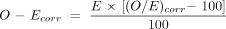
We adjusted for bias due to case mix as follows. The observed frequency (O) of each outcome in a unit was compared with the expected frequency (E). This can be expressed as a ratio (O/E) or as a difference (O–E). The difference can also be expressed as a percentage of the number of admissions (n) to give the so-called W score, where W = 100(O–E)/n. The crude (unadjusted) value of E is simply the overall rate for all units multiplied by n. The adjusted value of E for each unit is the sum of the predicted probabilities for all the infants in that unit, obtained from the logistic regression model to adjust for the five predictor variables. The crude and adjusted results were compared to show the effect of adjusting for case mix.
The gamma-Poisson hierarchical model was used to obtain the shrinkage estimators.10 These shrunken rates are less variable than the observed rates and provide a better estimate of a unit’s true rate. Details of this Bayesian approach are given in the Appendix. The model assumes that the units have rates that are exchangeable. Although it could be argued that the units actually differ so their rates are not exchangeable, in the absence of any unit covariates that could be included in the model there is no alternative but to assume exchangeability. Given this assumption, the results for all units are used to improve the estimate for each individual unit. The estimate for each unit shrinks towards the overall mean, with the shrinkage being greater for smaller units. The resulting estimates thus tend to be more conservative.11 The effect of using shrinkage estimators can be determined by comparing the estimates with and without this adjustment. The shrinkage can be applied to the incidence ratio O/E, the rate O/n, or the excess number of events O–E, as shown in the Appendix.
The frequency distributions of the observed and shrunken rates were plotted to show the variation in the rates and the effect of the shrinkage. However, these do not reveal whether there were large differences in the number of patients involved. A chart showing the shrunken excess O–E for each unit was therefore constructed and sorted by the number of patients in each unit to show whether there was a relationship between O–E and the number of admissions. On this chart the 95% limits are also shown to indicate the magnitude of the random variation for each unit.
Finally, we calculated the shrunken rate for the 20th centile. This figure represents the rate at or below which 20% of units are estimated to be operating. This may represent a realistic estimate of the “best practice” rate that could be achieved.10 The figure of 20% is used because it is approximately one standard deviation from the mean rate. If this is close to the overall rate, then all units are obtaining similar outcomes. If it is considerably less than the overall rate, there is evidence that the variation between units may have causes that could lead to improvement. The number of events that could be prevented if the overall rate were reduced to the 20th centile can then be determined.
RESULTS
The overall rate of severe IVH in the 24 NICUs was 6.8% for the 5413 infants with complete data on all five predictor variables. The reported rates for each individual unit are shown in column 4 of table 1; 50% of units reported rates between 5.7% and 8.1% (interquartile range, IQR). There were some extreme values in the rates of IVH, with the lowest at 2.9% and the highest over 20%. Figure 1A shows the observed rates and fig 1B shows the rates after adjusting for case mix, for which the IQR was increased to 5.9–9.7%. Column 5 of table 1 shows the shrunken rates without adjusting for case mix. The greater extent of change between the rates before and after shrinkage at both the lower and higher values shows that some of these extreme values may be due to random variation. A histogram of the shrunken rates looks as expected with a log normal or gamma distribution (fig 1C). Fifty percent of units had shrunken rates between 6.3% and 7.5%, with the extreme rates brought inwards to 4.0% and 11.6%.
Observed rates of severe IVH for 24 NICUs, and shrunken rates, unadjusted and adjusted for all five predictor variables in ascending order of observed rate of severe IVH
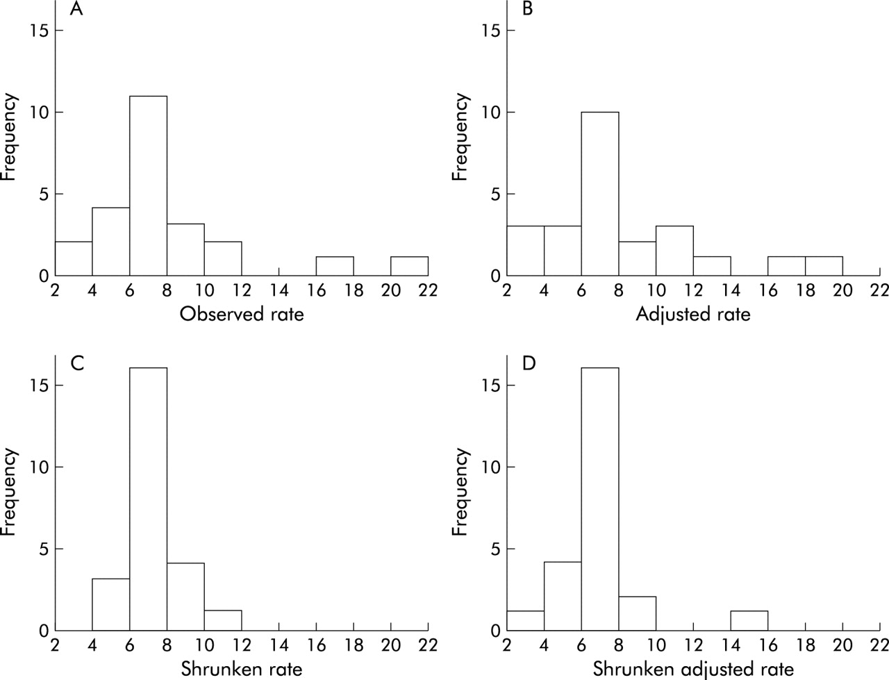
Histograms of rates of severe IVH showing (A) observed rates, (B) rates after adjusting for five predictor variables, (C) shrunken rates, and (D) shrunken adjusted rates.
Column 7 of table 1 shows the shrunken rates calculated after adjusting for differences in case mix using the five predictor variables. Fifty percent of units had shrunken rates corrected for case mix between 6.3% and 7.6%, with extremes of 3.8% and 14.2%. For these data, adjusting for case mix actually increased the spread of the rates among units rather than reducing or eliminating the differences, as can be seen by comparing figs 1A and 1B or 1C and 1D. The order of the units by rate was relatively unchanged using the shrinkage estimates, as shown in column 6 of table 1. Adjusting for the five predictors, however, had a more marked effect on the order, especially for units 5, 11, 16 and 19, although the five most extreme units did not change. The relative impact of the effects of adjusting for case mix and using shrinkage estimators is shown in fig 2.
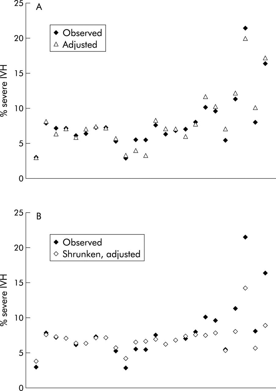
Observed percentage of cases with severe IVH in each unit, ordered from left to right by decreasing number of admissions, and (A) percentage adjusted for the five predictors but no shrinkage or (B) percentage adjusted for the five predictors and using shrunken estimates.
In table 2 the results using shrinkage estimators are compared with those obtained using W scores. First the expected number of cases of severe IVH (E) was calculated for each unit from the logistic regression equation adjusting for the five predictor variables. Shrunken O–E values were calculated using equation (1) and 95% limits using equation (2) in the Appendix. Use of shrunken estimates resulted in only the two most extreme units exceeding the 95% limits, unit 2 being significantly lower and unit 24 significantly higher than expected. In contrast, the use of W scores resulted in six units being declared significant at the 5% level.
Observed (O) and expected (E) cases of severe IVH for 24 NICUs, actual and shrunken estimates of excess cases (O–E), and W scores, adjusted for five predictor variables
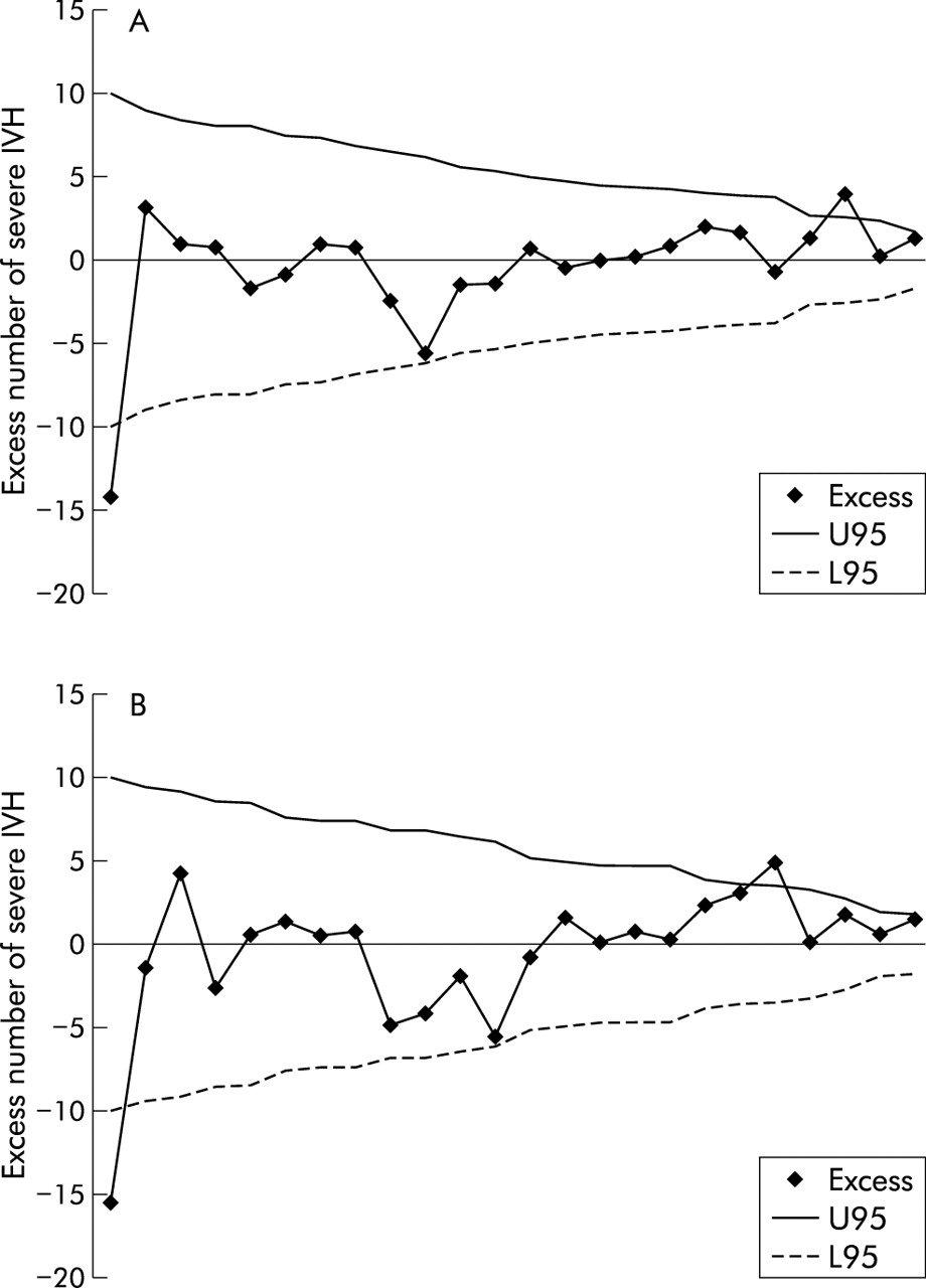
To determine how many patients were involved in creating the variation, fig 3A shows the observed minus the expected number of severe IVH cases for each unit, derived using the shrinkage estimates (see Appendix). The units are ordered by number of cases, the largest unit on the left and the smallest on the right. For most units O–E is close to zero with a maximum of 2–3 infants in excess or deficit in the 3 year period, although the largest unit had 16 fewer cases than expected. Although the histograms in fig 1 suggest that there are some outliers, fig 3A indicates that, individually, they are almost consistent with the expected amount of random variation. The plot for the results adjusted for the five predictor variables is very similar to that for the unadjusted results, as shown in fig 3B. Figure 3 also suggests that the excess of observed cases (O–E) increases as the number of cases in a unit decreases, the smallest 11 units all observing more cases than expected.
Excess number of severe IVH by unit (A) without adjusting for predictor variables and (B) after adjusting for the five predictor variables. Excess is O–E, calculated using shrunken estimators. U95 and L95 are upper and lower 95% control limits. Units are ordered by decreasing number of IVH cases expected, with the largest unit on the left.
However, there remains the variation between all units. Is it acceptable, or is there evidence of differences in clinical practice? The estimates (v) of the variation between the true rates of the units are given in table 3 for four scenarios in which the expected frequencies are unadjusted, and adjusted for three, four and five of the significant predictors. The values of v show that adjustment for case mix actually increased the estimate of between unit variation. However, the significance of this variation in terms of the number of cases of severe IVH that could be prevented is best quantified by using the 20th centile. Adjusting for all five predictors, the best 20% of units are estimated to have a rate of 5.74% or less, while the average is currently 6.84% (370/5413). If we could achieve an average rate of 5.74%, this would represent 60 (=5413 × (6.84 – 5.74)/100) fewer cases of severe IVH and a corresponding better outcome. This figure, in the final column of table 3, demonstrates most clearly the effect of adjusting for the significant predictors, despite the fact that variation due to the strongest predictor (the rate of complete steroid use) accounts for only about 8% of the variation in severe IVH rates.
Estimates of systematic variation between units in severe IVH rates, 20th centile rate, and number of cases that might be preventable
DISCUSSION
These data highlight the complex statistical problems involved in comparing clinical outcomes between hospitals. The ANZNN is a network of all the tertiary newborn intensive care units in Australia and New Zealand. In this region, very little intensive care for very preterm babies is provided outside these units, so these data are population based.
Intraventricular haemorrhage is one of the major morbidities of the very preterm baby and the more severe grades 3 and 4 are strongly associated with death or survival with disability. Because of this, reduction in rates of IVH is a clinical and research priority within neonatology. The analysis in this paper was stimulated by the wide variation in the rate of severe IVH between hospitals apparent in the raw data.8 If the organisational or clinical practice variables that were associated with the low rates in the best performing units could be identified, then it might be possible to reduce the rate of IVH across the whole network. In order to achieve that goal, it was necessary to allow for important identifiable sources of variation.
Measurement bias may well be an issue in this variation. The ANZNN tries to minimise measurement bias by having a strict set of definitions to which all units adhere. Before commencing this study, the directors of all the NICUs were surveyed to ensure they were using the agreed ultrasound classification of IVH. Despite this, there remains the possibility that some of the variation is due to measurement bias. To study this more closely, we are currently undertaking a retrospective independent audit of ultrasound scans across part of the network.
Case mix differences have been the dominant concern in the literature with respect to bias in outcome reporting. This study included a detailed analysis of predictive variables.8 It was an unexpected finding that, when the hospital outcome rates were adjusted for these variables, the spread of IVH rates increased rather than decreased. While for a few hospitals adjusting for case mix produced a large change in ranking, for the hospitals with the highest and lowest rates it made little difference. This observation may not be applicable to other populations or healthcare systems. Newborn intensive care is completely regionalised in Australia and New Zealand with very few babies born before 30 weeks being cared for outside the recognised tertiary centres. The result of this may be a more homogeneous case mix than in other healthcare systems.
Much more of the variation in IVH rates was due to sampling variability. This is particularly important because this variability will be greatest in the smallest units, making these units vulnerable in outcome comparisons that do not control for this source of variability. When these data were analysed using W scores, six units had severe IVH rates significantly different from the predicted rate. The four units with rates significantly higher than expected were all smaller units. When the data were adjusted for both case mix and sampling variability, only one of these units remained above the 95% limit. Further calculations show that this hospital is very close to the upper three-sigma limit. Three-sigma limits are used to adjust for the problem of multiple comparisons and are used by the Australian Council for Healthcare Standards for reporting clinical indicators in health care.16,17 This plot also quantifies the excess number of IVH cases observed at that hospital (n=5), which may be too few to warrant a quality improvement project to determine the possible causes. Continued monitoring would be appropriate for this possible quality problem. This analysis suggests that the variation across all units for this outcome is somewhat greater than expected by chance. The possibility that the excess number of cases increases as the unit size decreases also needs further exploration to determine whether there are any clinical causes.
How should this analysis be used to inform quality improvement? Often, after such comparisons, attention is focused on the hospitals with the worst outcome. However, one of the strengths of this analysis is that it quantifies the extent of random variation and gives an estimate of the improvement that can be expected by reducing the mean to that of the 20th centile. This information can be used to decide whether an intervention aimed at reducing the mean rate would be cost effective. It is instructive to note that, if the hospital with the highest rate were to reduce its rate of severe IVH to its expected rate, the result would be just five fewer cases of severe IVH over a 3 year period across the whole of Australia and New Zealand. In contrast, if we were to focus attention on the hospitals with rates below the 20th centile to find out what they are doing right, and if by applying those findings across the network the mean rate could be reduced to the current 20th centile, the result would be 60 fewer cases of severe IVH over a 3 year period in this region. This latter approach would seem more productive.
This study provides a method for reporting the quality of health care in NICUs in Australia and New Zealand. This method, which is also applicable to most quality of care indicators, has identified two aspects that were unexpected. The first was that adjusting for patient factors did not explain the variation between units, but actually increased the variation by almost 20%. The second was that, rather than revealing units with poor performance, there was more potential for improvement by reviewing the unit that had superior performance and determining the root causes of its better than average results. We suggest that these findings may occur in many similar studies, and that the current focus on case mix adjustment and identification of poor performance could be misplaced.
Key messages
-
Adjusting for differences in patient factors increased, rather than decreased, the variation between hospitals in rates of severe intraventricular haemorrhage (IVH) in very premature babies.
-
Shrinkage estimators were used to obtain better estimates of the true IVH rate for each hospital.
-
Greater reductions in morbidity may be achieved by concentrating on the best, rather than the worst, performing hospitals.
-
If factors that result in hospitals having lower morbidity rates could be identified, the overall average rate for all hospitals might be reduced.
Appendix: Calculation of rates and ratios using shrinkage estimators
Within each unit the random variation of the observed rate around the true rate is assumed to follow a Poisson distribution with mean = ei × λi, where ei is the expected number of cases in unit i and λi is the true underlying incidence ratio for unit i.10 Under a random effects (hierarchical) model, the units are assumed to be drawn from a population of such units. Their true incidence ratios, λi, are then assumed to have a gamma distribution with mean μ, which is close to 1, and standard deviation σ. An estimate v of σ and its approximate standard error (SE) are obtained from the data using maximum likelihood methods.18 Thus, v estimates the variation between units in their true rates. This estimate is then used to obtain the shrinkage estimators as follows.
The shrunken incidence ratio O/E (expressed as a percentage) is given by:

with standard error

The shrunken rate (expressed as a percentage) is given by:

with standard error

The shrunken rate for the 20th centile is estimated as simply the (n + 1)/5th value of the shrunken rates sorted in ascending order.
The shrunken excess O–E is calculated as:
The 95% limits are calculated from the Poisson distribution as ±U95, where

Acknowledgments
The authors thank Deborah Donoghue and members of the Australian and New Zealand Neonatal Network. We are grateful to the referee for helpful comments that improved this paper.